By Sarah Flood and Kamila Kolpashnikova
Time diary data: a unique opportunity
Time diary data offer researchers an opportunity to visualize daily life in a way that just isn’t possible with other data and demonstrating how people spend time. Respondents report every activity that they engage in (along with where and who they were with) over the course of the day, which means that time diaries can indicate how much time was spent in various activities as well as when activities occur during the day (e.g., timing) and the order in which they occur (i.e., sequencing) . This blog post will describe how to transform IPUMS ATUS data to perform these types of analyses, illustrate how to create a tempogram (including sample code), and link to additional resources for creating tempograms and performing sequence analysis.
While there are several ways to leverage the unique properties of time diary data, analysts are increasingly interested in creating tempograms and conducting sequence analyses, both of which capitalize on the temporal specificity of time diary data. These techniques allow researchers to explore the timing and order of activities over the course of a day. Both creating tempograms and conducting sequence analysis require time units that are consistent across respondents. Most time diary data are not natively in this format.
Data Preparation
Preparing the data for creating tempograms and conducting sequence analysis is labor-intensive, requiring substantial time investment and programming skill. Below, we provide users with guidance on how to use Stata and R to prepare the data for analyzing the rhythms of daily life. This requires completing a two-stage process of converting the data received from IPUMS ATUS into a long file where each record represents a one-minute interval and then into a wide file where the activity done during each minute of the day is represented as a minute-specific activity variable on a single record per person. This is one approach, though there are others (here is a description using R).
The shortest duration of a reported activity permitted in the American Time Use Survey (ATUS) is one minute, meaning that activities range in length from one minute to more than one thousand minutes. For this reason, most researchers creating tempograms will likely want to create a minute-level file for the ATUS where each ATUS respondent has 1,440 records representing each minute of the day. Once the data are in this format, the researcher can easily decide whether to use all 1,440 records per person or to select a subset of records.1 At this point the data are ready to be converted into a file where the activity performed each minute of the data is stored on a single record per person.
An Example
Our goal here is to illustrate how to produce a data file where each record represents a single individual whose 1440 minutes of the day are described on their record and generate a tempogram.
Step 1: Because there are 1,440 minutes in a day, each person’s time diary will be converted into 1,440 single-minute records. Getting the data into this format requires some manipulation. For the purposes of this example, we will describe the process using an IPUMS ATUS activity-level file2 (more information about this data format) where each activity reported by an ATUS respondent is represented by a separate record. It is critical to include the following variables in your data file: CASEID, ACTLINE, DURATION.
Here is a concrete example of what we’re trying to accomplish. An activity that represents five minutes spent cooking breakfast would be converted into five separate, one-minute records with each activity coded as cooking and a duration of one minute. Performing this operation across all ATUS respondents in 2021 (N=9,087) whose time diaries include 164,581 activity records yields a total of 13,085,280 records, each with a duration of one minute. Below is an example of syntax in Stata to perform this type of transformation on the data:
expand duration
bysort caseid (actline): gen seqactline=_n
gen seqduration=1
Step 2: With a minute-level file in hand, the data are then converted into the format needed to create figures like the tempograms below that shows at the population level how time is allocated to work, sleep, and other activities across the day or to conduct sequence analysis (resources provided below). Here are examples of syntax in R and Stata to perform this type of transformation on the data:
reshape wide activity, i(caseid) j(seqactline)
OR
collapse (mean) [activities categories of interest], by(seqactline)
Step 3: Generate a tempogram! The entire code needed to create this figure is found below, as is a similar example using R.
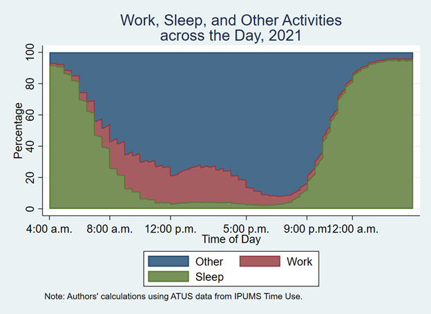
This tempogram demonstrates widespread norms of sleeping overnight and working during the day and illustrates a unique way to utilize and visualize time diary data. This tempogram shows the percentage of persons who report sleep in green, work in red, and other activities in blue. The x-axis is time of day, spanning the period from 4:00a.m. to 4:00a.m., and you can see most people are sleeping at 4:00am when the time diary begins, with the percentage persons reporting sleep at high levels overnight and lower during the day where work and other activities are higher. Time spent working is more concentrated (with highest rates from about 8:00am to 5:00pm) than other activities.
Tempograms often precede more sophisticated analyses such as sequence and cluster analysis. While tempograms are fun to create and analyze, they represent just a glimpse into what we can learn about the rhythms of daily life using these data. There is much more variation in the population in the patterns of daily life to describe and understand. This, however, is precisely the purpose of sequence analysis! We list some additional resources below that you may find useful for creating tempograms and conducting sequence analysis.
Resources
Tempograms
- Creating tempograms with ATUS data
- Kolpashnikova, K., Flood, S., et al. (2021). Exploring daily time-use patterns: ATUS-X data extractor and online diary visualization tool. PLoS One. Open access.
Sequence analysis
- Social Sequence Analysis (https://doi.org/10.1017/CBO9781316212530)
- SADI (https://www.stata-journal.com/article.html?article=st0486)
- TraMineR (http://traminer.unige.ch/)
- Sequence Analysis of ATUS-X data: Kolpashnikova, K. (2022, September 4). Sequence Analysis: Time Use Data (ATUS-X). https://doi.org/10.31219/osf.io/yt2gh
- Sequence Analysis Association bibliography (https://www.zotero.org/groups/2268769/saa_bibliography)
- Kolpashnikova, K., & Kan, M. Y. (2020). Eldercare in Japan: Cluster Analysis of daily time-use patterns of elder caregivers. Journal of Population Ageing, 1-23. (https://link.springer.com/article/10.1007/s12062-020-09313-3)
An example using R
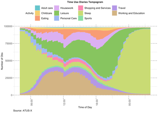
R code for generating the figure above
## load packages that we will be working with
library(ggplot2)
library(tidyverse)
library(paletteer)
library(grid)
library(gridExtra)
library(ipumsr)
## load timeuse package
devtools::install_github(“Kolpashnikova/package_R_timeuse”)
library(timeuse)
## Load ATUS-X extract
ddi <- read_ipums_ddi(“data/atus_00003.xml”)
data <- read_ipums_micro(ddi)
## find out which color palette you want to use
palettes_d_names
palettes_d_names %>% distinct(package)
view(palettes_d_names %>% filter(length>=12))
## transform data using tu_longtempo function
tem <- tu_longtempo(data, w = “WT06”)
## save as a dataframe
df <- as.data.frame(tem$values)
names(df) <- tem$key
## define time labels
t_intervals_labels <- seq.POSIXt(as.POSIXct(“2022-12-03 04:00:00 GMT”),
as.POSIXct(“2022-12-04 03:59:00 GMT”), by = “1 min”)
## add positions and time labels
df$time <- 1:1440
df$t_intervals_labels <- t_intervals_labels
## create a tempogram using ggplot
df %>%
gather(variable, value, Sleep:Travel) %>%
ggplot(aes(x = t_intervals_labels, y = value, fill = variable)) +
geom_area() +
scale_x_datetime(labels = scales::date_format(“%H:%M”, tz=”EST”)) +
#scale_fill_manual(values = paletteer_d(“RColorBrewer::Set3”,11)) +
scale_fill_manual(name = “Activity”, values = paletteer_d(“rcartocolor::Pastel”,11)) +
#coord_flip() +
labs(title = “Time Use Diaries Tempogram”,
x = “Time of Day”,
y = “Number of Obs”,
caption = “Source: ATUS-X”) +
theme(panel.background = element_blank(),
panel.grid.major = element_line(color = “grey20”, linetype = “dashed”),
panel.grid.minor = element_line(color = “grey10”, linetype = “dotted”),
plot.title = element_text(hjust = 0.5, face=”bold”, size = 14),
axis.text.x = element_text(angle=90, size = 14),
axis.text.y = element_text(size = 14),
axis.title.x = element_text(size = 14),
axis.title.y = element_text(size = 14),
plot.caption = element_text(hjust = 0, size = 14),
legend.position = “top”,
legend.key.size = unit(1, “cm”),
legend.text = element_text(size = 14),
legend.title = element_text(size = 14))
Full Stata Code for Creating Tempogram
expand duration
bysort caseid (actline): gen seqactline=_n
gen seqduration=1
gen act=3
replace act=1 if activity==10101
replace act=2 if activity>=050000 & sf_activity<050400
gen sleep=(act==1)
gen work=(act==2)
gen other=(act==3)
collapse (mean) sleep work other, by(seqactline)
replace sleep=sleep*100
replace work=work*100
replace other=other*100
replace work=sleep+work
replace other=100
twoway area other seqactline || area work seqactline || area sleep seqactline, legend(order(1 “Other” 2 “Work” 3 “Sleep”)) ytitle(Percentage) xtitle(Time of Day) xlab(1 “4:00 a.m.” 240 “8:00 a.m.” 480 “12:00 p.m.” 780 “5:00 p.m.” 1020 “9:00 p.m.” 1200 “12:00 a.m.”) title(“Work, Sleep, and Other Activities” “across the Day, 2021”) note(“Note: Authors’ calculations using ATUS data from IPUMS Time Use.”)