By Divya Pandey and Anna Bolgrien
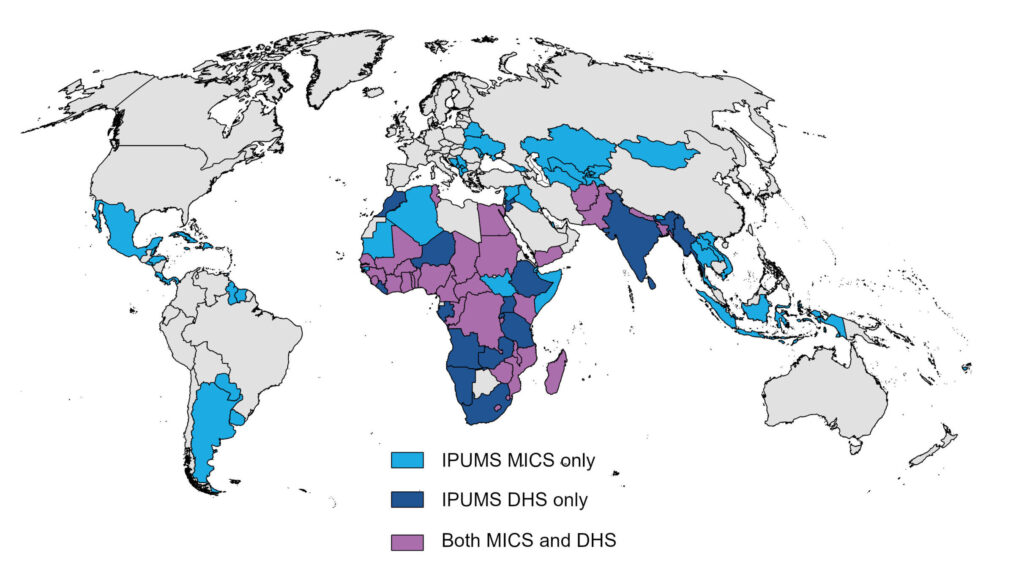
In a research project combining data from IPUMS MICS and IPUMS DHS, IPUMS Global Health staff examined trends in the relationship between open defecation and high infant mortality rates (IMR) in the Eastern Indo-Gangetic Plains. The project focused on selected bordering regions in Nepal, Bangladesh, and India. By analyzing these environmentally and agro-climatically comparable regions, the study aimed to isolate the impact of national and local policies on open defecation and infant mortality rates.
Figure 1: Regions included in the study

The study pooled data from IPUMS MICS and IPUMS DHS to look at trends over almost two decades. IPUMS DHS includes data for all three countries, and IPUMS MICS provides additional years of data for Nepal and Bangladesh. Since the study focused on selected bordering geographies, the authors worked with data from lower administrative levels—divisions in Bangladesh, states in India, and regions in Nepal. Leveraging the geography resources provided by IPUMS, the team used both spatially harmonized and sample-specific geography variables (learn more about IPUMS DHS geography variables and IPUMS MICS geography variables). Spatially harmonized geography variables identify geographic regions using a consistent spatial footprint to allow for the comparison of the same physical space over time. Sample-specific geography variables are not harmonized across time; as their name suggests, they use the geographic boundaries that are sample-specific or contemporaneous to the survey-year in a country.